Extreme (Xarray): computing EFI and SOT

In this notebook you will see how to:

• compute the Extreme Forecast Index (EFI) from Xarray data

• plot the resulting EFI field

• compute the Shift of Tails (SOT) as a complement to EFI

We will use earthkit-data for getting the input data and earthkit-plots for plotting.

import earthkit.data as ekd
import earthkit.plots as ekp

from earthkit.meteo import extreme

Getting the data

The sample forecast contains ensemble 2 m temperature data and the second sample contains the corresponding model-climate information. EFI and SOT compare the forecast distribution against that model climate for the same parameter, lead time and time of year.

ds_fc = ekd.from_source("sample", "extreme_2t_fc.grib").to_xarray()
ds_fc

<xarray.Dataset> Size: 347MB
Dimensions:    (member: 101, values: 421120)
Coordinates:
  * member     (member) <U3 1kB '0' '1' '10' '100' '11' ... '96' '97' '98' '99'
    latitude   (values) float64 3MB ...
    longitude  (values) float64 3MB ...
Dimensions without coordinates: values
Data variables:
    2t         (member, values) float64 340MB ...
Attributes:
    Conventions:  CF-1.8
    institution:  ECMWF

xarray.Dataset

• Dimensions:
  • member: 101
  • values: 421120
• Coordinates: (3)
  • member
    (member)
    <U3
    '0' '1' '10' ... '97' '98' '99'

    standard_name :

    realization

    long_name :

    ensemble member id

    array(['0', '1', '10', '100', '11', '12', '13', '14', '15', '16', '17', '18',
           '19', '2', '20', '21', '22', '23', '24', '25', '26', '27', '28', '29',
           '3', '30', '31', '32', '33', '34', '35', '36', '37', '38', '39', '4',
           '40', '41', '42', '43', '44', '45', '46', '47', '48', '49', '5', '50',
           '51', '52', '53', '54', '55', '56', '57', '58', '59', '6', '60', '61',
           '62', '63', '64', '65', '66', '67', '68', '69', '7', '70', '71', '72',
           '73', '74', '75', '76', '77', '78', '79', '8', '80', '81', '82', '83',
           '84', '85', '86', '87', '88', '89', '9', '90', '91', '92', '93', '94',
           '95', '96', '97', '98', '99'], dtype='<U3')

  • latitude
    (values)
    float64
    ...

    units :

    degrees_north

    standard_name :

    latitude

    long_name :

    latitude

    [421120 values with dtype=float64]

  • longitude
    (values)
    float64
    ...

    units :

    degrees_east

    standard_name :

    longitude

    long_name :

    longitude

    [421120 values with dtype=float64]

• Data variables: (1)
  • 2t
    (member, values)
    float64
    ...

    standard_name :

    unknown

    long_name :

    2 metre temperature

    units :

    kelvin

    level_type :

    surface

    _earthkit :

    {"message": {"__bytes_b64__": "R1JJQgAFogEAAGqAYp7/gKcBAAAaAwoAAAEAqAMAHAAVAAAAAAAAAAAAAAAAAAAAHgFQBGIwMDAxAGUCAAAAAAAAAAAAAAAAAAAAAAAAAAAAAAAAAAAAAAAAAAAAAAAAAAAAAAAAAAAAAAAAAAAAAAAAAAUgACEE//8CgAFeuAAAAACBXrgFfSr//wFAAAAAAAAAFAAYABwAIAAkACgALAAwADQAOAA8AEAARABIAEwAUABUAFgAXABgAGQAaABsAHAAdAB4AHwAgACEAIgAjACQAJQAmACcAKAApACoAKwAsAC0ALgAvADAAMQAyADMANAA1ADYANwA4ADkAOgA7ADwAPQA+AD8AQABBAEIAQwBEAEUARgBHAEgASQBKAEsATABNAE4ATwBQAFEAUgBTAFQAVQBWAFcAWABZAFoAWwBcAF0AXgBfAGAAYQBiAGMAZABlAGYAZwBoAGkAagBrAGwAbQBuAG8AcABxAHIAcwB0AHUAdgB3AHgAeQB6AHsAfAB9AH4AfwCAAIEAggCDAIQAhQCGAIcAiACJAIoAiwCMAI0AjgCPAJAAkQCSAJMAlACVAJYAlwCYAJkAmgCbAJwAnQCeAJ8AoAChAKIAowCkAKUApgCnAKgAqQCqAKsArACtAK4ArwCwALEAsgCzALQAtQC2ALcAuAC5ALoAuwC8AL0AvgC/AMAAwQDCAMMAxADFAMYAxwDIAMkAygDLAMwAzQDOAM8A0ADRANIA0wDUANUA1gDXANgA2QDaANsA3ADdAN4A3wDgAOEA4gDjAOQA5QDmAOcA6ADpAOoA6wDsAO0A7gDvAPAA8QDyAPMA9AD1APYA9wD4APkA+gD7APwA/QD+AP8BAAEBAQIBAwEEAQUBBgEHAQgBCQEKAQsBDAENAQ4BDwEQAREBEgETARQBFQEWARcBGAEZARoBGwEcAR0BHgEfASABIQEiASMBJAElASYBJwEoASkBKgErASwBLQEuAS8BMAExATIBMwE0ATUBNgE3ATgBOQE6ATsBPAE9AT4BPwFAAUEBQgFDAUQBRAFDAUIBQQFAAT8BPgE9ATwBOwE6ATkBOAE3ATYBNQE0ATMBMgExATABLwEuAS0BLAErASoBKQEoAScBJgElASQBIwEiASEBIAEfAR4BHQEcARsBGgEZARgBFwEWARUBFAETARIBEQEQAQ8BDgENAQwBCwEKAQkBCAEHAQYBBQEEAQMBAgEBAQAA/wD+AP0A/AD7APoA+QD4APcA9gD1APQA8wDyAPEA8ADvAO4A7QDsAOsA6gDpAOgA5wDmAOUA5ADjAOIA4QDgAN8A3gDdANwA2wDaANkA2ADXANYA1QDUANMA0gDRANAAzwDOAM0AzADLAMoAyQDIAMcAxgDFAMQAwwDCAMEAwAC/AL4AvQC8ALsAugC5ALgAtwC2ALUAtACzALIAsQCwAK8ArgCtAKwAqwCqAKkAqACnAKYApQCkAKMAogChAKAAnwCeAJ0AnACbAJoAmQCYAJcAlgCVAJQAkwCSAJEAkACPAI4AjQCMAIsAigCJAIgAhwCGAIUAhACDAIIAgQCAAH8AfgB9AHwAewB6AHkAeAB3AHYAdQB0AHMAcgBxAHAAbwBuAG0AbABrAGoAaQBoAGcAZgBlAGQAYwBiAGEAYABfAF4AXQBcAFsAWgBZAFgAVwBWAFUAVABTAFIAUQBQAE8ATgBNAEwASwBKAEkASABHAEYARQBEAEMAQgBBAEAAPwA+AD0APAA7ADoAOQA4ADcANgA1ADQAMwAyADEAMAAvAC4ALQAsACsAKgApACgAJwAmACUAJAAjACIAIQAgAB8AHgAdABwAGwAaABkAGAAXABYAFQAUABMAEgARABAADwAOAA0ADAALAAoACQAIAAcABgAFAAADACAAkS5fW4AADc3Nzc="}, "bitsPerValue": 16}

    [42533120 values with dtype=float64]

• Attributes: (2)

  Conventions :

  CF-1.8

  institution :

  ECMWF

Next, we load the model-climate data used as the reference distribution.

ds_clim = ekd.from_source("sample", "extreme_2t_clim.grib").to_xarray()
ds_clim

<xarray.Dataset> Size: 347MB
Dimensions:    (member: 101, values: 421120)
Coordinates:
  * member     (member) <U3 1kB '0' '1' '10' '100' '11' ... '96' '97' '98' '99'
    latitude   (values) float64 3MB ...
    longitude  (values) float64 3MB ...
Dimensions without coordinates: values
Data variables:
    avg_2t     (member, values) float64 340MB ...
Attributes:
    Conventions:  CF-1.8
    institution:  ECMWF

xarray.Dataset

• Dimensions:
  • member: 101
  • values: 421120
• Coordinates: (3)
  • member
    (member)
    <U3
    '0' '1' '10' ... '97' '98' '99'

    standard_name :

    realization

    long_name :

    ensemble member id

    array(['0', '1', '10', '100', '11', '12', '13', '14', '15', '16', '17', '18',
           '19', '2', '20', '21', '22', '23', '24', '25', '26', '27', '28', '29',
           '3', '30', '31', '32', '33', '34', '35', '36', '37', '38', '39', '4',
           '40', '41', '42', '43', '44', '45', '46', '47', '48', '49', '5', '50',
           '51', '52', '53', '54', '55', '56', '57', '58', '59', '6', '60', '61',
           '62', '63', '64', '65', '66', '67', '68', '69', '7', '70', '71', '72',
           '73', '74', '75', '76', '77', '78', '79', '8', '80', '81', '82', '83',
           '84', '85', '86', '87', '88', '89', '9', '90', '91', '92', '93', '94',
           '95', '96', '97', '98', '99'], dtype='<U3')

  • latitude
    (values)
    float64
    ...

    units :

    degrees_north

    standard_name :

    latitude

    long_name :

    latitude

    [421120 values with dtype=float64]

  • longitude
    (values)
    float64
    ...

    units :

    degrees_east

    standard_name :

    longitude

    long_name :

    longitude

    [421120 values with dtype=float64]

• Data variables: (1)
  • avg_2t
    (member, values)
    float64
    ...

    standard_name :

    unknown

    long_name :

    Time-mean 2 metre temperature

    units :

    kelvin

    level_type :

    surface

    _earthkit :

    {"message": {"__bytes_b64__": "R1JJQgAFiAEAAFDkYp7/gAQBAAAaAwsAAAEAqAMAHAAVAAAAAAAAAAAAAAAAAAAAEwEgBGEwMDAxAGRPATTa2AAAFAAABwAETAAAAAAAAAAAAAAAAAAAAAAFIAAhBP//AoABXrgAAAAAgV64BX0q//8BQAAAAAAAABQAGAAcACAAJAAoACwAMAA0ADgAPABAAEQASABMAFAAVABYAFwAYABkAGgAbABwAHQAeAB8AIAAhACIAIwAkACUAJgAnACgAKQAqACsALAAtAC4ALwAwADEAMgAzADQANQA2ADcAOAA5ADoAOwA8AD0APgA/AEAAQQBCAEMARABFAEYARwBIAEkASgBLAEwATQBOAE8AUABRAFIAUwBUAFUAVgBXAFgAWQBaAFsAXABdAF4AXwBgAGEAYgBjAGQAZQBmAGcAaABpAGoAawBsAG0AbgBvAHAAcQByAHMAdAB1AHYAdwB4AHkAegB7AHwAfQB+AH8AgACBAIIAgwCEAIUAhgCHAIgAiQCKAIsAjACNAI4AjwCQAJEAkgCTAJQAlQCWAJcAmACZAJoAmwCcAJ0AngCfAKAAoQCiAKMApAClAKYApwCoAKkAqgCrAKwArQCuAK8AsACxALIAswC0ALUAtgC3ALgAuQC6ALsAvAC9AL4AvwDAAMEAwgDDAMQAxQDGAMcAyADJAMoAywDMAM0AzgDPANAA0QDSANMA1ADVANYA1wDYANkA2gDbANwA3QDeAN8A4ADhAOIA4wDkAOUA5gDnAOgA6QDqAOsA7ADtAO4A7wDwAPEA8gDzAPQA9QD2APcA+AD5APoA+wD8AP0A/gD/AQABAQECAQMBBAEFAQYBBwEIAQkBCgELAQwBDQEOAQ8BEAERARIBEwEUARUBFgEXARgBGQEaARsBHAEdAR4BHwEgASEBIgEjASQBJQEmAScBKAEpASoBKwEsAS0BLgEvATABMQEyATMBNAE1ATYBNwE4ATkBOgE7ATwBPQE+AT8BQAFBAUIBQwFEAUQBQwFCAUEBQAE/AT4BPQE8ATsBOgE5ATgBNwE2ATUBNAEzATIBMQEwAS8BLgEtASwBKwEqASkBKAEnASYBJQEkASMBIgEhASABHwEeAR0BHAEbARoBGQEYARcBFgEVARQBEwESAREBEAEPAQ4BDQEMAQsBCgEJAQgBBwEGAQUBBAEDAQIBAQEAAP8A/gD9APwA+wD6APkA+AD3APYA9QD0APMA8gDxAPAA7wDuAO0A7ADrAOoA6QDoAOcA5gDlAOQA4wDiAOEA4ADfAN4A3QDcANsA2gDZANgA1wDWANUA1ADTANIA0QDQAM8AzgDNAMwAywDKAMkAyADHAMYAxQDEAMMAwgDBAMAAvwC+AL0AvAC7ALoAuQC4ALcAtgC1ALQAswCyALEAsACvAK4ArQCsAKsAqgCpAKgApwCmAKUApACjAKIAoQCgAJ8AngCdAJwAmwCaAJkAmACXAJYAlQCUAJMAkgCRAJAAjwCOAI0AjACLAIoAiQCIAIcAhgCFAIQAgwCCAIEAgAB/AH4AfQB8AHsAegB5AHgAdwB2AHUAdABzAHIAcQBwAG8AbgBtAGwAawBqAGkAaABnAGYAZQBkAGMAYgBhAGAAXwBeAF0AXABbAFoAWQBYAFcAVgBVAFQAUwBSAFEAUABPAE4ATQBMAEsASgBJAEgARwBGAEUARABDAEIAQQBAAD8APgA9ADwAOwA6ADkAOAA3ADYANQA0ADMAMgAxADAALwAuAC0ALAArACoAKQAoACcAJgAlACQAIwAiACEAIAAfAB4AHQAcABsAGgAZABgAFwAWABUAFAATABIAEQAQAA8ADgANAAwACwAKAAkACAAHAAYABQAAAwAgAJEuX1uAAA3Nzc3"}, "bitsPerValue": 12}

    [42533120 values with dtype=float64]

• Attributes: (2)

  Conventions :

  CF-1.8

  institution :

  ECMWF

Extreme Forecast Index

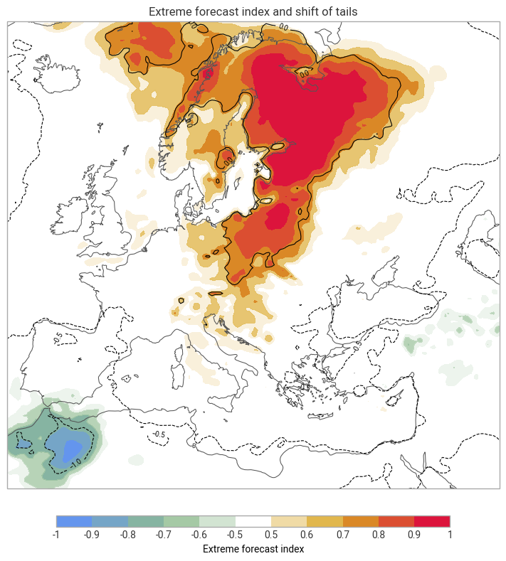
EFI measures how unusual the ensemble forecast distribution is relative to model climate. ECMWF defines it from the difference between the forecast and model-climate cumulative distribution functions, with extra weight given to the tails of the distribution. EFI values lie between -1 and 1. In practice, EFI values around 0.5 to 0.8 often indicate unusual conditions, while values above about 0.8 suggest very unusual or extreme conditions. For 2 m temperature, positive EFI highlights unusually warm conditions and negative EFI highlights unusually cold conditions.

References: ECMWF Forecast User Guide: EFI and SOT overview, ECMWF Forecast User Guide: calculating EFI, Introducing earthkit.

We compute EFI with efi() using the forecast temperature field and the average 2 m temperature model-climate field.

efi = extreme.efi(ds_clim["avg_2t"], ds_fc["2t"])

Finally, we plot the EFI field to identify the regions where the forecast departs most strongly from model climate. This version keeps the custom map styling added in the concurrent changes.

efi_style = ekp.styles.Style(
    levels=[-1, -0.9, -0.8, -0.7, -0.6, -0.5, 0.5, 0.6, 0.7, 0.8, 0.9, 1],
    colors=["cornflowerblue", "darkseagreen", (1, 1, 1, 0), "goldenrod", "crimson"],
)

chart = ekp.Map(domain="Europe")

chart.contourf(
    efi,
    style=efi_style,
)

chart.coastlines()
chart.title("Extreme forecast index")
chart.legend(label="Extreme forecast index")

chart.show()

Shift of Tails

SOT complements EFI. ECMWF notes that EFI alone does not distinguish between ensemble members that merely reach the model-climate extreme and members that go well beyond it. SOT was introduced to describe how far the forecast tail extends relative to model climate. In the upper tail, ECMWF defines SOT from the 90th and 99th percentiles of the ensemble and model-climate distributions. Positive SOT indicates that at least 10% of the ensemble is forecasting an extreme event.

Reference: ECMWF Forecast User Guide: calculating SOT.

The example below uses the same forecast and climate inputs as for the EFI. We use the sot() method to compute the SOT.

sot = extreme.sot(ds_clim["avg_2t"], ds_fc["2t"], 90)

As with EFI, a quick plot is useful for checking where the most pronounced tail shifts are located. We overlay SOT with the previously computed EFI.

chart = ekp.Map(domain="Europe")

chart.contour(
    sot,
    levels=[-2, -1.5, -1, -0.5, 0, 0.5, 1],
    # levels=[0, 1, 2, 5, 8],
    colors="black",
    linewidths=0.8,
    legend_style=None,
)

chart.contourf(efi, style=efi_style)

chart.coastlines()
chart.title("Extreme forecast index and shift of tails")
chart.legend(label="Extreme forecast index")

chart.show()