Fieldlist: Interpolating from hybrid to height levels
This notebook demonstrates how to interpolate GRIB fieldlist data on hybrid model levels to height levels. We will use two different methods:
interpolate_hybrid_to_height_levels(). This is a convenience method dedicated to this particular interpolation.interpolate_monotonic(). This is a generic method and requires an extra step to compute the height on hybrid levels, which then it can be applied to multiple interpolations.
We will use earthkit-data for fieldlist support and earthkit-plots for plotting.
[1]:
import earthkit.data as ekd
import earthkit.plots as ekp
import numpy as np

import earthkit.meteo.vertical.fieldlist as vertical
Hybrid levels
Hybrid levels are terrain following at the bottom and isobaric at the top of the atmosphere with a transition in between. This is the vertical coordinate system in the IFS model.
For details about the hybrid levels see [IFS-CY49R1-Dynamics] Chapter 2, Section 2.2.1. Also see the /how-tos/vertical/hybrid_levels_grib.ipynb notebook for the related computations in earthkit-meteo.
Getting the data
The input is GRIB data on 137 IFS model levels for one step. We fetch the file and extract temperature, specific humidity, the surface geopotential and the log surface pressure.
[2]:
fl = ekd.from_source("sample", "tq_ml137_europe.grib2").to_fieldlist()

# LNSP → surface pressure [Pa]
lnsp = fl.sel({"parameter.variable": "lnsp", "vertical.level": 1})[0]
sp = lnsp.set(values=np.exp(lnsp.values))

t = fl.sel({"parameter.variable": "t"})  # temperature, 137 levels
q = fl.sel({"parameter.variable": "q"})  # specific humidity, 137 levels
zs = fl.sel({"parameter.variable": "z", "vertical.level": 1})[0]  # surface geopotential

t.head()
[2]:
| parameter.variable | time.valid_datetime | time.base_datetime | time.step | vertical.level | vertical.level_type | ensemble.member | geography.grid_type | |
|---|---|---|---|---|---|---|---|---|
| 0 | t | 2019-06-02 12:00:00 | 2019-06-02 12:00:00 | 0 days | 1 | hybrid | None | regular_ll |
| 1 | t | 2019-06-02 12:00:00 | 2019-06-02 12:00:00 | 0 days | 2 | hybrid | None | regular_ll |
| 2 | t | 2019-06-02 12:00:00 | 2019-06-02 12:00:00 | 0 days | 3 | hybrid | None | regular_ll |
| 3 | t | 2019-06-02 12:00:00 | 2019-06-02 12:00:00 | 0 days | 4 | hybrid | None | regular_ll |
| 4 | t | 2019-06-02 12:00:00 | 2019-06-02 12:00:00 | 0 days | 5 | hybrid | None | regular_ll |
Please note that although lnsp and z are valid for the surface in our data they are available on hybrid level 1. This is how IFS forecast and analysis data is stored in ECMWF’s MARS archive (from where our the data is originating).
The A and B coefficients defining the hybrid levels are embedded in the field metadata and are inferred automatically.
Using interpolate_hybrid_to_height_levels
interpolate_hybrid_to_height_levels() interpolates data from hybrid levels to a set of target heights (m). The height type and reference level are controlled by h_type and h_reference.
Target: geometric height above the ground
[3]:
target_h = [1000.0, 5000.0]  # geometric height (m), above the ground

t_res = vertical.interpolate_hybrid_to_height_levels(
    t,  # data to interpolate
    target_h,
    t,  # temperature for height computation
    q,  # specific humidity for height computation
    zs,  # surface geopotential
    sp,  # surface pressure
    h_type="geometric",
    h_reference="ground",
    interpolation="linear",
)
t_res.ls()
[3]:
| parameter.variable | time.valid_datetime | time.base_datetime | time.step | vertical.level | vertical.level_type | ensemble.member | geography.grid_type | |
|---|---|---|---|---|---|---|---|---|
| 0 | t | 2019-06-02 12:00:00 | 2019-06-02 12:00:00 | 0 days | 1000.0 | height_above_ground_level | None | regular_ll |
| 1 | t | 2019-06-02 12:00:00 | 2019-06-02 12:00:00 | 0 days | 5000.0 | height_above_ground_level | None | regular_ll |
[4]:
# the first 2 values from the resulting fields
t_res.values[:, :2]
[4]:
array([[268.9916733 , 269.2149941 ],
       [246.53155411, 246.83113775]])
[5]:
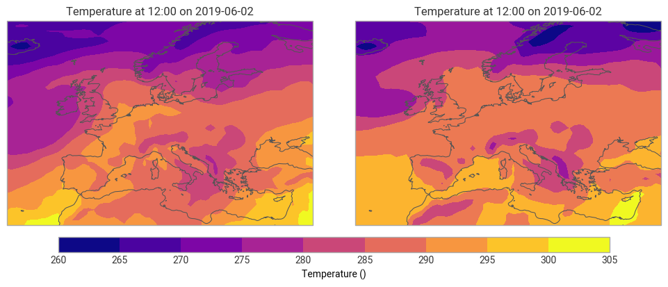
# plot the resulting fields
ekp.quickplot(t_res)
[5]:
<earthkit.plots.components.figures.Figure at 0x10ee93b60>
Target: geometric height above sea level
[6]:
target_h_sea = [1000.0, 5000.0]  # geometric height (m), above sea level

t_res_sea = vertical.interpolate_hybrid_to_height_levels(
    t,
    target_h_sea,
    t,
    q,
    zs,
    sp,
    h_type="geometric",
    h_reference="sea",
    interpolation="linear",
)
t_res_sea.ls()
[6]:
| parameter.variable | time.valid_datetime | time.base_datetime | time.step | vertical.level | vertical.level_type | ensemble.member | geography.grid_type | |
|---|---|---|---|---|---|---|---|---|
| 0 | t | 2019-06-02 12:00:00 | 2019-06-02 12:00:00 | 0 days | 1000.0 | height_above_mean_sea_level | None | regular_ll |
| 1 | t | 2019-06-02 12:00:00 | 2019-06-02 12:00:00 | 0 days | 5000.0 | height_above_mean_sea_level | None | regular_ll |
[7]:
# the first 2 values from the resulting fields
t_res_sea.values[:, :2]
[7]:
array([[268.94972844, 269.35456355],
       [246.48962616, 246.96957874]])
Target: geopotential height above the ground
[8]:
target_h_gp = [1000.0, 5000.0]  # geopotential height (m), above the ground

t_res_gp = vertical.interpolate_hybrid_to_height_levels(
    t,
    target_h_gp,
    t,
    q,
    zs,
    sp,
    h_type="geopotential",
    h_reference="ground",
    interpolation="linear",
)
t_res_gp.ls()
[8]:
| parameter.variable | time.valid_datetime | time.base_datetime | time.step | vertical.level | vertical.level_type | ensemble.member | geography.grid_type | |
|---|---|---|---|---|---|---|---|---|
| 0 | t | 2019-06-02 12:00:00 | 2019-06-02 12:00:00 | 0 days | 1000.0 | height_above_ground_level | None | regular_ll |
| 1 | t | 2019-06-02 12:00:00 | 2019-06-02 12:00:00 | 0 days | 5000.0 | height_above_ground_level | None | regular_ll |
[9]:
# the first 2 values from the resulting fields
t_res_gp.values[:, :2]
[9]:
array([[268.99075524, 269.21401367],
       [246.50819277, 246.80779845]])
Using a subset of levels
It is possible to use only a subset of the model levels in the input data. This can significantly speed up the computations and reduce memory usage. The model level range must be contiguous and include the bottom-most level.
Unfortunately, the model level height is not constant (changing with gridpoint and time) and to determine which subset we need we have to find the lowest model level that is entirely above the highest target height. This computation is almost as costly as the interpolation itself so to avoid it we typically use a guess. E.g. if we want to interpolate data to heights of 1000 and 5000 m above ground level the lowest 50 model levels should be enough. For the sake of this exercise we check the validity of this assumption for the current data with height_on_hybrid_levels(). The computation shows that model level 88 lies entirely higher than 5000 m above ground, so our assumption was correct.
[10]:
levels = list(range(88, 138))
t_bot = t.sel({"vertical.level": levels})
q_bot = q.sel({"vertical.level": levels})

h_sub = vertical.height_on_hybrid_levels(t_bot, q_bot, zs, sp, h_type="geometric", h_reference="ground")

# the minimum height on model level 88
h_sub[0].values.min()
[10]:
np.float64(6950.382024204814)
Now we perform the interpolation by using only the lowest 50 model levels.
[11]:
# keep only the 50 lowest model levels
t_sub = t.sel({"vertical.level": list(range(88, 138))})
q_sub = q.sel({"vertical.level": list(range(88, 138))})

t_res_sub = vertical.interpolate_hybrid_to_height_levels(
    t_sub,
    target_h,
    t_sub,
    q_sub,
    zs,
    sp,
    h_type="geometric",
    h_reference="ground",
    interpolation="linear",
)
t_res_sub.ls()
[11]:
| parameter.variable | time.valid_datetime | time.base_datetime | time.step | vertical.level | vertical.level_type | ensemble.member | geography.grid_type | |
|---|---|---|---|---|---|---|---|---|
| 0 | t | 2019-06-02 12:00:00 | 2019-06-02 12:00:00 | 0 days | 1000.0 | height_above_ground_level | None | regular_ll |
| 1 | t | 2019-06-02 12:00:00 | 2019-06-02 12:00:00 | 0 days | 5000.0 | height_above_ground_level | None | regular_ll |
[12]:
# the first 2 values from the resulting fields
t_res_gp.values[:, :2]
[12]:
array([[268.99075524, 269.21401367],
       [246.50819277, 246.80779845]])
Using aux levels
The lowest (full) model level is always above the surface (its height changing with gridpoint and time). Therefore, interpolation to a height between the surface and the lowest model level returns NaN. We can compute the height of the lowest model level with height_on_hybrid_levels() to see this gap.
[13]:
t_bottom = t.sel({"vertical.level": [137]})
q_bottom = q.sel({"vertical.level": [137]})

# height of the bottom level above ground (m)
h_bottom = vertical.height_on_hybrid_levels(t_bottom, q_bottom, zs, sp, h_type="geometric", h_reference="ground")

# plot the field
ekp.quickplot(h_bottom)
[13]:
<earthkit.plots.components.maps.Map at 0x129134690>
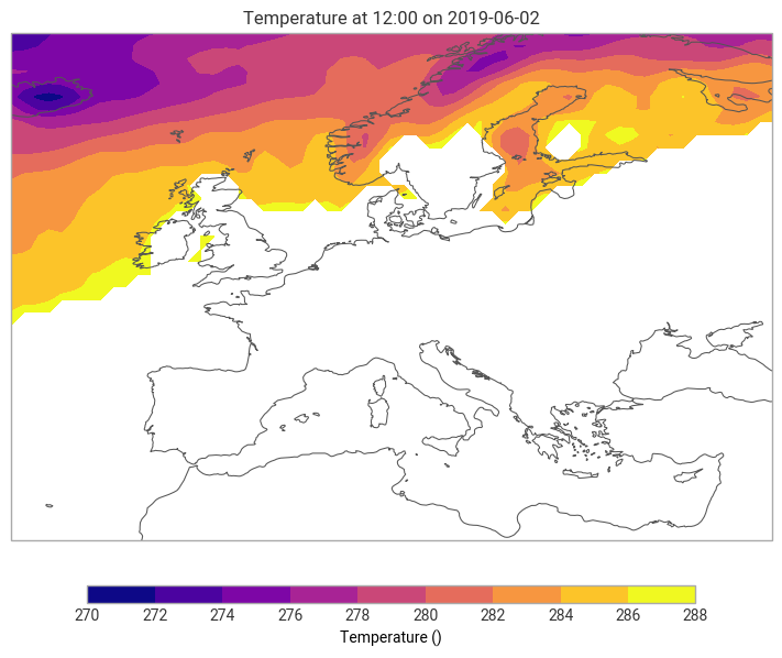
We can see that the lowest model level is approximately 10 m above the ground, at many gridpoints higher than 10 m. Interpolating to 10 m therefore yields NaN at all these locations.
[14]:
target_h_near_surf = [10.0]  # m above the ground

t_res_nan = vertical.interpolate_hybrid_to_height_levels(
    t,
    target_h_near_surf,
    t,
    q,
    zs,
    sp,
    h_type="geometric",
    h_reference="ground",
    interpolation="linear",
)

# plot the result
ekp.quickplot(t_res_nan)
[14]:
<earthkit.plots.components.maps.Map at 0x129140510>
To overcome this problem we can supply auxiliary data via the aux_bottom_h and aux_bottom_data kwargs. Both can be a single value (constant) or a field. As a demonstration, we simply set the temperature at height 0 m (the surface) to slightly higher than at the lowest model level.
[15]:
t_res_aux = vertical.interpolate_hybrid_to_height_levels(
    t,
    target_h_near_surf,
    t,
    q,
    zs,
    sp,
    h_type="geometric",
    h_reference="ground",
    aux_bottom_h=0.0,  # m — height of the auxiliary level (surface)
    aux_bottom_data=t[-1] + 0.06,  # K — set field as temperature at the surface
    interpolation="linear",
)

# plot the resulting field
ekp.quickplot(t_res_aux)
[15]:
<earthkit.plots.components.maps.Map at 0x1291415b0>

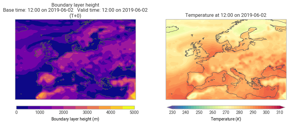
Interpolating to a height field
The target height in interpolate_hybrid_to_height_levels() can also be a field/fieldlist, with changing target in each gridpoint. To demonstrate this we interpolate the temperature to the height of the boundary layer. First, we fetch the boundary layer height field for the same date and time as our input data.
[16]:
blh = ekd.from_source("sample", "blh_europe.grib1").to_fieldlist()[0]
blh.ls()
[16]:
| parameter.variable | time.valid_datetime | time.base_datetime | time.step | vertical.level | vertical.level_type | ensemble.member | geography.grid_type | |
|---|---|---|---|---|---|---|---|---|
| 0 | blh | 2019-06-02 12:00:00 | 2019-06-02 12:00:00 | 0 days | 0 | surface | 0 | regular_ll |
This field contains heights above ground, so we need to set h_reference="ground" for the interpolation.
[17]:
t_res_blh = vertical.interpolate_hybrid_to_height_levels(
    t,
    blh,
    t,
    q,
    zs=zs,
    sp=sp,
    h_type="geometric",
    h_reference="ground",
    interpolation="linear",
)
t_res_blh.ls()
[17]:
| parameter.variable | time.valid_datetime | time.base_datetime | time.step | vertical.level | vertical.level_type | ensemble.member | geography.grid_type | |
|---|---|---|---|---|---|---|---|---|
| 0 | t | 2019-06-02 12:00:00 | 2019-06-02 12:00:00 | 0 days | 315.217041 | height_above_ground_level | None | regular_ll |
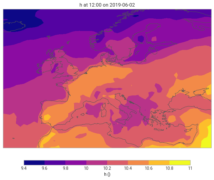
We plot the boundary layer height and the temperature interpolated to it side by side.
[18]:
ekp.quickplot(ekd.FieldList.from_fields([blh, t_res_blh]))
[18]:
<earthkit.plots.components.figures.Figure at 0x129142b10>

Using interpolate_monotonic
We can also use interpolate_monotonic() to carry out the interpolation. This is a generic method and requires an extra step to compute the height on (full) model levels using height_on_hybrid_levels(). Then this height data can be reused to interpolate multiple fieldlists. This can be the main advantage over interpolate_hybrid_to_height_levels(), which needs to compute the height (internally) on hybrid levels on each call.
Target: geometric height above the ground
First, compute the geometric height above the ground on all the model levels in the input data. The height type and reference level are controlled by h_type and h_reference.
[19]:
h = vertical.height_on_hybrid_levels(t, q, zs, sp, h_type="geometric", h_reference="ground")
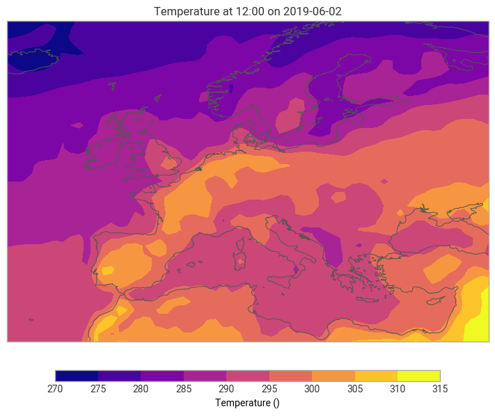
Next, interpolate the temperature to the target height levels.
[20]:
target_h = [1000.0, 5000.0]  # geometric height (m), above the ground

t_res = vertical.interpolate_monotonic(
    t, coord=h, target_coord=target_h, coord_type="height_above_ground_level", interpolation="linear"
)
t_res.ls()
[20]:
| parameter.variable | time.valid_datetime | time.base_datetime | time.step | vertical.level | vertical.level_type | ensemble.member | geography.grid_type | |
|---|---|---|---|---|---|---|---|---|
| 0 | t | 2019-06-02 12:00:00 | 2019-06-02 12:00:00 | 0 days | 1000.0 | height_above_ground_level | None | regular_ll |
| 1 | t | 2019-06-02 12:00:00 | 2019-06-02 12:00:00 | 0 days | 5000.0 | height_above_ground_level | None | regular_ll |
[21]:
# the first 2 values from the resulting fields
t_res.values[:, :2]
[21]:
array([[268.9916733 , 269.2149941 ],
       [246.53155411, 246.83113775]])
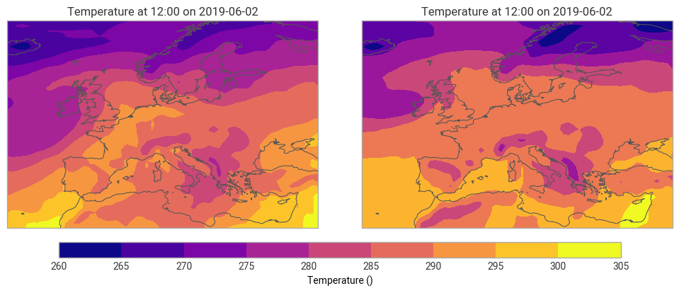
[22]:
# plot the resulting fields
ekp.quickplot(t_res)
[22]:
<earthkit.plots.components.figures.Figure at 0x1291fc830>
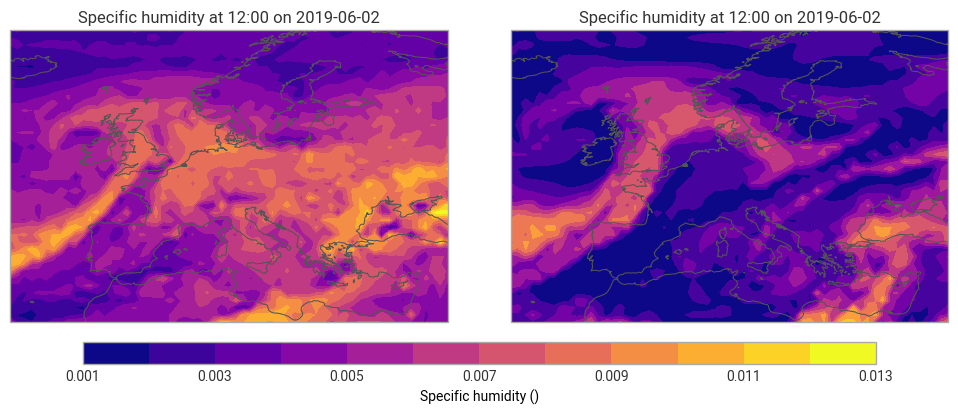
The same computation is repeated with specific humidity (notice that we reused the height fieldlist).
[23]:
q_res = vertical.interpolate_monotonic(
    q, coord=h, target_coord=target_h, coord_type="height_above_ground_level", interpolation="linear"
)
q_res.ls()
[23]:
| parameter.variable | time.valid_datetime | time.base_datetime | time.step | vertical.level | vertical.level_type | ensemble.member | geography.grid_type | |
|---|---|---|---|---|---|---|---|---|
| 0 | q | 2019-06-02 12:00:00 | 2019-06-02 12:00:00 | 0 days | 1000.0 | height_above_ground_level | None | regular_ll |
| 1 | q | 2019-06-02 12:00:00 | 2019-06-02 12:00:00 | 0 days | 5000.0 | height_above_ground_level | None | regular_ll |
[24]:
# the first 2 values from the resulting fields
q_res.values[:, :2]
[24]:
array([[0.00279257, 0.00303697],
       [0.00049974, 0.0005222 ]])
[25]:
# plot the resulting fields
ekp.quickplot(q_res)
[25]:
<earthkit.plots.components.figures.Figure at 0x12c09a9c0>
Target: geometric height above sea level
[26]:
target_h_sea = [1000.0, 5000.0]  # geometric height (m), above sea level

h_sea = vertical.height_on_hybrid_levels(t, q, zs, sp, h_type="geometric", h_reference="sea")

t_res_sea = vertical.interpolate_monotonic(
    t, coord=h_sea, target_coord=target_h, coord_type="height_above_sea_level", interpolation="linear"
)
t_res_sea.ls()
[26]:
| parameter.variable | time.valid_datetime | time.base_datetime | time.step | vertical.level | vertical.level_type | ensemble.member | geography.grid_type | |
|---|---|---|---|---|---|---|---|---|
| 0 | t | 2019-06-02 12:00:00 | 2019-06-02 12:00:00 | 0 days | 1000.0 | height_above_sea_level | None | regular_ll |
| 1 | t | 2019-06-02 12:00:00 | 2019-06-02 12:00:00 | 0 days | 5000.0 | height_above_sea_level | None | regular_ll |
[27]:
# the first 2 values from the resulting fields
t_res_sea.values[:, :2]
[27]:
array([[268.94972844, 269.35456355],
       [246.48962616, 246.96957874]])
Target: geopotential height above the ground
[28]:
target_h_gp = [1000.0, 5000.0]  # geopotential height (m), above the ground

h_gp = vertical.height_on_hybrid_levels(t, q, zs, sp, h_type="geopotential", h_reference="ground")

t_res_gp = vertical.interpolate_monotonic(
    t, coord=h_gp, target_coord=target_h, coord_type="height_above_ground_level", interpolation="linear"
)
t_res_gp.ls()
[28]:
| parameter.variable | time.valid_datetime | time.base_datetime | time.step | vertical.level | vertical.level_type | ensemble.member | geography.grid_type | |
|---|---|---|---|---|---|---|---|---|
| 0 | t | 2019-06-02 12:00:00 | 2019-06-02 12:00:00 | 0 days | 1000.0 | height_above_ground_level | None | regular_ll |
| 1 | t | 2019-06-02 12:00:00 | 2019-06-02 12:00:00 | 0 days | 5000.0 | height_above_ground_level | None | regular_ll |
[29]:
# the first 2 values from the resulting fields
t_res_sea.values[:, :2]
[29]:
array([[268.94972844, 269.35456355],
       [246.48962616, 246.96957874]])
Using a subset of levels
It is possible to use only a subset of the model levels in the input data. This can significantly speed up the computations and reduce memory usage. The model level range must be contiguous and include the bottom-most level.
Unfortunately, the model level height is not constant (changing with gridpoint and time) and to determine which subset we need we have to find the lowest model level that is entirely above the highest target height. To avoid the excessive computations we can use a guess for it. E.g. if we want to interpolate data to heights of 1000 and 5000 m above ground level the lowest 50 model levels should be enough. The height is already computed for all the levels in this notebook so we can check the validity of this assumption for the current data. We can see that model level 88 lies entirely higher than 5000 m above ground, so our assumption was correct.
[30]:
h[87].values.min()
[30]:
np.float64(6950.382024204814)
Now we perform the interpolation by using only the lowest 50 model levels.
[31]:
# keep only the 50 lowest model levels
t_sub = t.sel({"vertical.level": list(range(88, 138))})
q_sub = q.sel({"vertical.level": list(range(88, 138))})

h_sub = vertical.height_on_hybrid_levels(t_sub, q_sub, zs, sp, h_type="geometric", h_reference="ground")

t_res_sub = vertical.interpolate_monotonic(
    t_sub, coord=h_sub, target_coord=target_h, coord_type="height_above_ground_level", interpolation="linear"
)
t_res_sub.ls()
[31]:
| parameter.variable | time.valid_datetime | time.base_datetime | time.step | vertical.level | vertical.level_type | ensemble.member | geography.grid_type | |
|---|---|---|---|---|---|---|---|---|
| 0 | t | 2019-06-02 12:00:00 | 2019-06-02 12:00:00 | 0 days | 1000.0 | height_above_ground_level | None | regular_ll |
| 1 | t | 2019-06-02 12:00:00 | 2019-06-02 12:00:00 | 0 days | 5000.0 | height_above_ground_level | None | regular_ll |
[32]:
# the first 2 values from the resulting fields
t_res_sub.values[:, :2]
[32]:
array([[268.9916733 , 269.2149941 ],
       [246.53155411, 246.83113775]])
Using aux levels
The lowest (full) model level is always above the surface. Therefore, interpolation to a height between the surface and the lowest model level returns NaN. The plot below shows the height (above ground) of the lowest model level.
[33]:
ekp.quickplot(h[-1])
[33]:
<earthkit.plots.components.maps.Map at 0x129656250>

We can see that the lowest model level is approximately 10 m above the ground, at many gridpoints higher than 10 m. Interpolating to 10 m therefore yields NaN at all these locations.
[34]:
target_h_near_surf = [10.0]  # m above the ground

t_res_nan = vertical.interpolate_monotonic(
    t, coord=h, target_coord=target_h_near_surf, coord_type="height_above_ground_level", interpolation="linear"
)

# plot the result
ekp.quickplot(t_res_nan)
[34]:
<earthkit.plots.components.maps.Map at 0x129655550>

To overcome this problem we can supply auxiliary data via the aux_min_level_coord and aux_min_level_data kwargs. Both can be a single value (constant) or a field. The example below simply set the temperature at height 0 m (the surface) to slightly higher than at the lowest model level. With this the interpolation works.
[35]:
t_res_aux = vertical.interpolate_monotonic(
    t,
    coord=h,
    target_coord=target_h_near_surf,
    coord_type="height_above_ground_level",
    aux_min_level_coord=0.0,  # m — height of the auxiliary level (surface)
    aux_min_level_data=t[-1] + 0.06,  # K — set field as temperature at the surface
    interpolation="linear",
)

# the first 2 values from the resulting fields
t_res_aux.values[:, :2]
[35]:
array([[273.57876195, 273.15646884]])
[36]:
# plot the resulting field
ekp.quickplot(t_res_aux)
[36]:
<earthkit.plots.components.maps.Map at 0x129657950>
Interpolating to a height field
The target height in interpolate_monotonic() can also be a field/fieldlist, with changing target in each gridpoint. To demonstrate this we interpolate the temperature to the height of the boundary layer. We will use the blh field fetched earlier in this notebook.
This field contains heights above ground, so we need to set h_reference="ground" for the interpolation.
[37]:
t_res_blh = vertical.interpolate_monotonic(
    t, coord=h, target_coord=blh, coord_type="height_above_ground_level", interpolation="linear"
)
t_res_blh.ls()
[37]:
| parameter.variable | time.valid_datetime | time.base_datetime | time.step | vertical.level | vertical.level_type | ensemble.member | geography.grid_type | |
|---|---|---|---|---|---|---|---|---|
| 0 | t | 2019-06-02 12:00:00 | 2019-06-02 12:00:00 | 0 days | 315.217041 | height_above_ground_level | None | regular_ll |
We plot the boundary layer height and the temperature interpolated to it side by side.
[38]:
ekp.quickplot(ekd.FieldList.from_fields([blh, t_res_blh]))
[38]:
<earthkit.plots.components.figures.Figure at 0x1291869c0>
Writing to GRIB
Currently, fieldlist based computations resulting in fieldlist keeping all the values in memory. We can save this data to GRIB with to_target.
[39]:
t_res.to_target("file", "_hybrid_to_hl.grib")

# read back and verify
t_res_saved = ekd.from_source("file", "_hybrid_to_hl.grib").to_fieldlist()
t_res_saved.ls()
[39]:
| parameter.variable | time.valid_datetime | time.base_datetime | time.step | vertical.level | vertical.level_type | ensemble.member | geography.grid_type | |
|---|---|---|---|---|---|---|---|---|
| 0 | t | 2019-06-02 12:00:00 | 2019-06-02 12:00:00 | 0 days | 1000 | height_above_ground_level | None | regular_ll |
| 1 | t | 2019-06-02 12:00:00 | 2019-06-02 12:00:00 | 0 days | 5000 | height_above_ground_level | None | regular_ll |
[40]:
# the first 2 values from the saved fields
t_res_saved.values[:, :2]
[40]:
array([[268.99203491, 269.21469116],
       [246.53132629, 246.83113098]])