Fieldlist: Interpolating from hybrid to pressure levels

This notebook demonstrates how to interpolate GRIB fieldlist data on hybrid model levels to height levels with interpolate_hybrid_to_pressure_levels(). We will use earthkit-data for fieldlist support and earthkit-plots for plotting.

import earthkit.data as ekd
import earthkit.plots as ekp
import numpy as np

import earthkit.meteo.vertical.fieldlist as vertical

Hybrid levels

Hybrid levels are terrain following at the bottom and isobaric at the top of the atmosphere with a transition in between. This is the vertical coordinate system in the IFS model.

For details about the hybrid levels see [IFS-CY49R1-Dynamics] Chapter 2, Section 2.2.1. Also see the /how-tos/vertical/hybrid_levels_grib.ipynb notebook for the related computations in earthkit-meteo.

Getting the data

The input is GRIB data on 137 IFS model levels for one step. We fetch the file and extract temperature, specific humidity and the log surface pressure.

fl = ekd.from_source("sample", "tq_ml137_europe.grib2").to_fieldlist()

# LNSP → surface pressure [Pa]
lnsp = fl.sel({"parameter.variable": "lnsp", "vertical.level": 1})[0]
sp = lnsp.set(values=np.exp(lnsp.values))

t = fl.sel({"parameter.variable": "t"})  # temperature, 137 levels
q = fl.sel({"parameter.variable": "q"})  # specific humidity, 137 levels

t.head()

	parameter.variable	time.valid_datetime	time.base_datetime	time.step	vertical.level	vertical.level_type	ensemble.member	geography.grid_type
0	t	2019-06-02 12:00:00	2019-06-02 12:00:00	0 days	1	hybrid	None	regular_ll
1	t	2019-06-02 12:00:00	2019-06-02 12:00:00	0 days	2	hybrid	None	regular_ll
2	t	2019-06-02 12:00:00	2019-06-02 12:00:00	0 days	3	hybrid	None	regular_ll
3	t	2019-06-02 12:00:00	2019-06-02 12:00:00	0 days	4	hybrid	None	regular_ll
4	t	2019-06-02 12:00:00	2019-06-02 12:00:00	0 days	5	hybrid	None	regular_ll

Please note that although lnsp is valid for the surface in our data it is available on hybrid level 1. This is how IFS forecast and analysis data is stored in ECMWF’s MARS archive (from where our the data is originating).

The A and B coefficients defining the hybrid levels are embedded in the GRIB metadata and are inferred automatically.

Using interpolate_hybrid_to_pressure_levels

interpolate_hybrid_to_pressure_levels() interpolates data from hybrid levels to a set of target pressure levels (Pa).

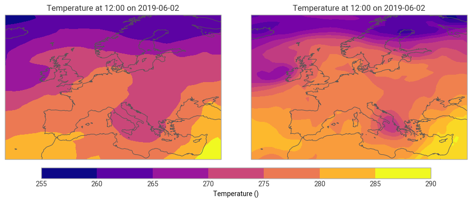
target_p = [70000.0, 50000.0]  # Pa

t_res = vertical.interpolate_hybrid_to_pressure_levels(
    t,  # data to interpolate
    target_p,
    sp,
    interpolation="linear",
)
t_res.ls()

	parameter.variable	time.valid_datetime	time.base_datetime	time.step	vertical.level	vertical.level_type	ensemble.member	geography.grid_type
0	t	2019-06-02 12:00:00	2019-06-02 12:00:00	0 days	700.0	pressure	None	regular_ll
1	t	2019-06-02 12:00:00	2019-06-02 12:00:00	0 days	500.0	pressure	None	regular_ll

# the first 2 values from the resulting fields
t_res.values[:, :2]

array([[256.7211221 , 257.00983999],
       [244.06243185, 244.50014912]])

# plot the resulting fields
ekp.quickplot(t_res)

<earthkit.plots.components.figures.Figure at 0x126e2bb60>

Using a subset of levels

It is possible to use only a subset of the model levels in the input data. This can significantly speed up the computations and reduce memory usage. The model level range must be contiguous and include the bottom-most level.

Unfortunately, the model level pressure is not constant (changing with gridpoint and time) and to determine which subset we need we have to find the lowest model level that is entirely above the lowest target pressure. We can use a guess for it. for it. E.g. if we want to interpolate data to pressures of 70000 and 50000 Pa the lowest 50 model levels should be enough. For the sake of this exercise we check the validity of this assumption for the current data with pressure_on_hybrid_levels(). The computation shows that the entire model level 88 lies higher than the 50000 Pa isosurface, so our assumption was correct.

p_sub = vertical.pressure_on_hybrid_levels(sp, levels=[88], output="full")

# the max pressure on model level 88
p_sub[0].values.max()

np.float64(36971.49325737165)

Now we perform the interpolation by using only the lowest 50 model levels.

# keep only the 50 lowest model levels
t_sub = t.sel({"vertical.level": list(range(88, 138))})

t_res_sub = vertical.interpolate_hybrid_to_pressure_levels(
    t_sub,
    target_p,
    sp,
    interpolation="linear",
)
t_res_sub.ls()

	parameter.variable	time.valid_datetime	time.base_datetime	time.step	vertical.level	vertical.level_type	ensemble.member	geography.grid_type
0	t	2019-06-02 12:00:00	2019-06-02 12:00:00	0 days	700.0	pressure	None	regular_ll
1	t	2019-06-02 12:00:00	2019-06-02 12:00:00	0 days	500.0	pressure	None	regular_ll

# the first value from the resulting fields
t_res.values[:, 0]

array([256.7211221 , 244.06243185])

Interpolating to a pressure field

The target pressure in interpolate_hybrid_to_pressure_levels() can also be a field/fieldlist, with changing target in each gridpoint. To demonstrate this we interpolate the temperature to the pressure of the 2 PVU potential vorticity level. First, we fetch this field for the same date and time as our input data.

pres_pv = ekd.from_source("sample", "pressure_on_pv_europe.grib1").to_fieldlist()[0]
pres_pv.ls()

	parameter.variable	time.valid_datetime	time.base_datetime	time.step	vertical.level	vertical.level_type	ensemble.member	geography.grid_type
0	pres	2019-06-02 12:00:00	2019-06-02 12:00:00	0 days	2000	potential_vorticity	0	regular_ll

Next, we interpolate the data to the target field.

t_res_pv = vertical.interpolate_hybrid_to_pressure_levels(
    t,
    pres_pv,
    sp,
    interpolation="linear",
)

t_res_pv.ls()

	parameter.variable	time.valid_datetime	time.base_datetime	time.step	vertical.level	vertical.level_type	ensemble.member	geography.grid_type
0	t	2019-06-02 12:00:00	2019-06-02 12:00:00	0 days	431.157539	pressure	None	regular_ll

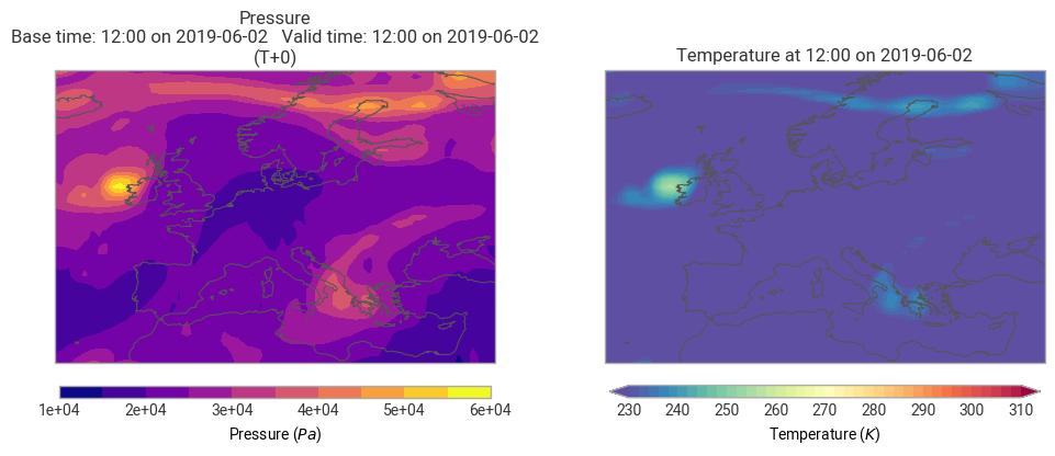
Finally, plot the pressure of the 2 PVU potential vorticity level and the temperature interpolated to it side by side.

ekp.quickplot(ekd.FieldList.from_fields([pres_pv, t_res_pv]))

<earthkit.plots.components.figures.Figure at 0x1698bb750>

Writing to GRIB

The resulting FieldList keeps all the values in memory. We can save the data to GRIB with to_target.

t_res.to_target("file", "_hybrid_to_pl.grib")

# read back and verify
ekd.from_source("file", "_hybrid_to_pl.grib").to_fieldlist().ls()

	parameter.variable	time.valid_datetime	time.base_datetime	time.step	vertical.level	vertical.level_type	ensemble.member	geography.grid_type
0	t	2019-06-02 12:00:00	2019-06-02 12:00:00	0 days	7	pressure	None	regular_ll
1	t	2019-06-02 12:00:00	2019-06-02 12:00:00	0 days	5	pressure	None	regular_ll