Fieldlist: Interpolating from pressure to height levels
This notebook demonstrates how to interpolate GRIB fieldlist data on pressure levels to height levels with interpolate_pressure_to_height_levels(). We will use earthkit-data for fieldlist support and earthkit-plots for plotting.
[1]:
import earthkit.data as ekd
import earthkit.plots as ekp

import earthkit.meteo.vertical.fieldlist as vertical
Getting the data
The input is GRIB data on pressure levels plus some surface fields. We fetch the file and inspect its contents.
[2]:
fl = ekd.from_source("sample", "tz_pl_global.grib1").to_fieldlist()
fl.head()
[2]:
| parameter.variable | time.valid_datetime | time.base_datetime | time.step | vertical.level | vertical.level_type | ensemble.member | geography.grid_type | |
|---|---|---|---|---|---|---|---|---|
| 0 | t | 2019-06-02 12:00:00 | 2019-06-02 12:00:00 | 0 days | 1000 | pressure | 0 | regular_ll |
| 1 | z | 2019-06-02 12:00:00 | 2019-06-02 12:00:00 | 0 days | 1000 | pressure | 0 | regular_ll |
| 2 | t | 2019-06-02 12:00:00 | 2019-06-02 12:00:00 | 0 days | 850 | pressure | 0 | regular_ll |
| 3 | z | 2019-06-02 12:00:00 | 2019-06-02 12:00:00 | 0 days | 850 | pressure | 0 | regular_ll |
| 4 | t | 2019-06-02 12:00:00 | 2019-06-02 12:00:00 | 0 days | 700 | pressure | 0 | regular_ll |
We will use the following fields from the file for interpolation:
t – temperature (K) on 12 pressure levels (1000, 850, 700, 500, 400, 300, 200, 150, 100, 70, 50, 30 hPa)
z – geopotential (m²/s²) on the same 12 pressure levels and on the surface
We extract each quantity below.
[3]:
t = fl.sel({"parameter.variable": "t", "vertical.level_type": "pressure"})
z = fl.sel({"parameter.variable": "z", "vertical.level_type": "pressure"})
zs = fl.sel({"parameter.variable": "z", "vertical.level_type": "surface"})[0]  # surface geopotential

t.head()
[3]:
| parameter.variable | time.valid_datetime | time.base_datetime | time.step | vertical.level | vertical.level_type | ensemble.member | geography.grid_type | |
|---|---|---|---|---|---|---|---|---|
| 0 | t | 2019-06-02 12:00:00 | 2019-06-02 12:00:00 | 0 days | 1000 | pressure | 0 | regular_ll |
| 1 | t | 2019-06-02 12:00:00 | 2019-06-02 12:00:00 | 0 days | 850 | pressure | 0 | regular_ll |
| 2 | t | 2019-06-02 12:00:00 | 2019-06-02 12:00:00 | 0 days | 700 | pressure | 0 | regular_ll |
| 3 | t | 2019-06-02 12:00:00 | 2019-06-02 12:00:00 | 0 days | 500 | pressure | 0 | regular_ll |
| 4 | t | 2019-06-02 12:00:00 | 2019-06-02 12:00:00 | 0 days | 400 | pressure | 0 | regular_ll |
Using interpolate_pressure_to_height_levels
interpolate_pressure_to_height_levels() interpolates data from pressure levels to a set of target heights (m). The function requires geopotential on the same pressure levels as the input data, and optionally the surface geopotential for ground-referenced heights.
Target: geometric height above the ground
[4]:
target_h = [1000.0, 5000.0]  # geometric height (m), above the ground

t_res = vertical.interpolate_pressure_to_height_levels(
    t,  # data on pressure levels to interpolate
    target_h,
    z,  # geopotential on the same pressure levels
    zs=zs,  # surface geopotential
    h_type="geometric",
    h_reference="ground",
    interpolation="linear",
)
t_res.ls()
[4]:
| parameter.variable | time.valid_datetime | time.base_datetime | time.step | vertical.level | vertical.level_type | ensemble.member | geography.grid_type | |
|---|---|---|---|---|---|---|---|---|
| 0 | t | 2019-06-02 12:00:00 | 2019-06-02 12:00:00 | 0 days | 1000.0 | height_above_ground_level | 0 | regular_ll |
| 1 | t | 2019-06-02 12:00:00 | 2019-06-02 12:00:00 | 0 days | 5000.0 | height_above_ground_level | 0 | regular_ll |
[5]:
# the first 2 values from the resulting fields
t_res.values[:, :2]
[5]:
array([[269.52995877, 269.52995877],
       [249.7430541 , 249.7430541 ]])
[6]:
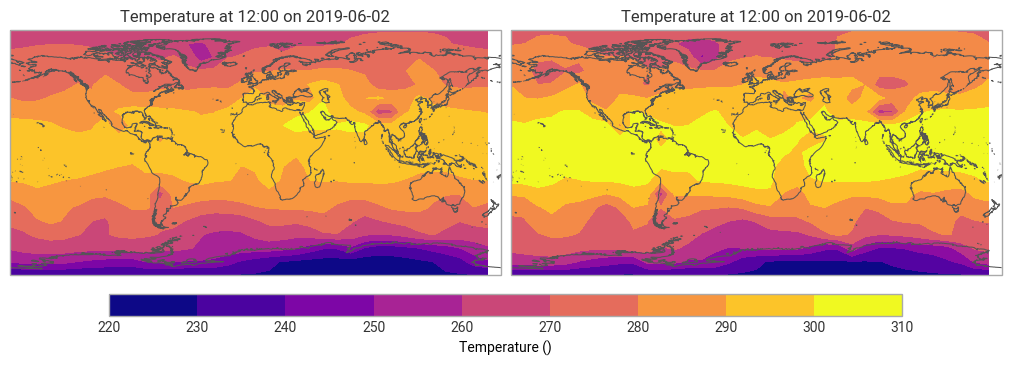
# plot the resulting fields
ekp.quickplot(t_res)
[6]:
<earthkit.plots.components.figures.Figure at 0x12f7b9d30>
Target: geometric height above sea level
[7]:
target_h_sea = [1000.0, 5000.0]  # geometric height (m), above sea level

# zs is not used when h_reference="sea"
t_res_sea = vertical.interpolate_pressure_to_height_levels(
    t,
    target_h_sea,
    z,
    h_type="geometric",
    h_reference="sea",
    interpolation="linear",
)
t_res_sea.ls()
[7]:
| parameter.variable | time.valid_datetime | time.base_datetime | time.step | vertical.level | vertical.level_type | ensemble.member | geography.grid_type | |
|---|---|---|---|---|---|---|---|---|
| 0 | t | 2019-06-02 12:00:00 | 2019-06-02 12:00:00 | 0 days | 1000.0 | height_above_mean_sea_level | 0 | regular_ll |
| 1 | t | 2019-06-02 12:00:00 | 2019-06-02 12:00:00 | 0 days | 5000.0 | height_above_mean_sea_level | 0 | regular_ll |
[8]:
# the first 2 values from the resulting fields
t_res_sea.values[:, :2]
[8]:
array([[269.53030875, 269.53030875],
       [249.74390207, 249.74390207]])
Target: geopotential height above the ground
[9]:
target_h_gp = [1000.0, 5000.0]  # geopotential height (m), above the ground

t_res_gp = vertical.interpolate_pressure_to_height_levels(
    t,
    target_h_gp,
    z,
    zs=zs,
    h_type="geopotential",
    h_reference="ground",
    interpolation="linear",
)
t_res_gp.ls()
[9]:
| parameter.variable | time.valid_datetime | time.base_datetime | time.step | vertical.level | vertical.level_type | ensemble.member | geography.grid_type | |
|---|---|---|---|---|---|---|---|---|
| 0 | t | 2019-06-02 12:00:00 | 2019-06-02 12:00:00 | 0 days | 1000.0 | height_above_ground_level | 0 | regular_ll |
| 1 | t | 2019-06-02 12:00:00 | 2019-06-02 12:00:00 | 0 days | 5000.0 | height_above_ground_level | 0 | regular_ll |
[10]:
# the first 2 values from the resulting fields
t_res_gp.values[:, :2]
[10]:
array([[269.52940015, 269.52940015],
       [249.7167234 , 249.7167234 ]])
Using aux levels
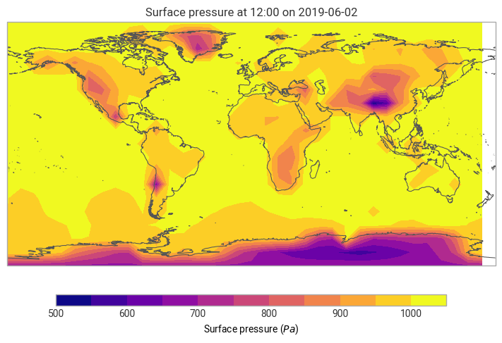
The lowest pressure level in the input data is 1000 hPa. In grid points where the surface pressure is significantly higher than 1000 hPa interpolation to near surface heights will result in NaNs. We can see these areas in the surface pressure plot.
[11]:
# extract and plot surface pressure (and convert to hPa for plotting)
sp = fl.sel({"parameter.variable": "sp"})[0] / 100.0
ekp.quickplot(sp)
[11]:
<earthkit.plots.components.maps.Map at 0x13c51fd90>
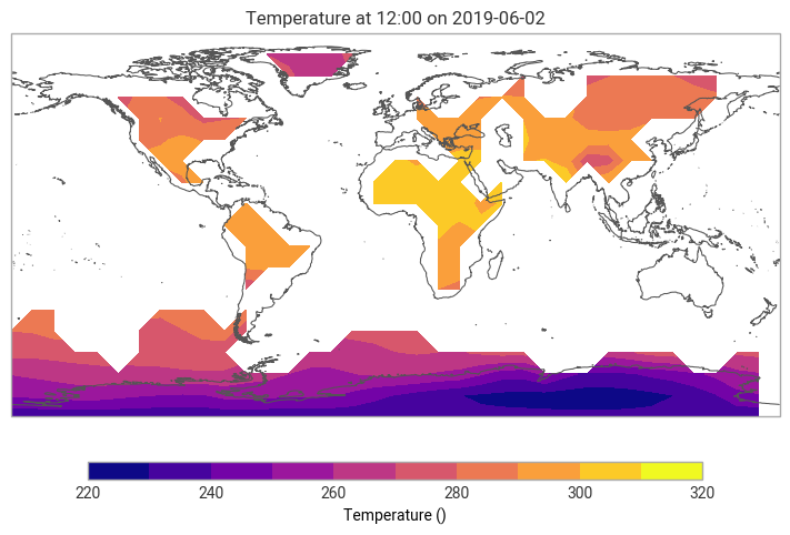
[12]:
target_h_near_surf = [10.0]  # m above the ground

t_res_nan = vertical.interpolate_pressure_to_height_levels(
    t,
    target_h_near_surf,
    z,
    zs=zs,
    h_type="geometric",
    h_reference="ground",
    interpolation="linear",
)

# plot the resulting fields
ekp.quickplot(t_res_nan)
[12]:
<earthkit.plots.components.maps.Map at 0x13e32dcd0>
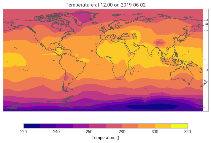
To overcome this problem we can supply auxiliary data via the aux_bottom_* kwargs. In the example below we use the 2m temperature field (available in the input data) as an auxiliary data. Note that the auxiliary data must be provided on a target coordinate level (height in this case).
[13]:
# extract 2m temperature field
t2 = fl.sel({"parameter.variable": "2t"})[0]

t_res_aux = vertical.interpolate_pressure_to_height_levels(
    t,
    target_h_near_surf,
    z,
    zs=zs,
    h_type="geometric",
    h_reference="ground",
    aux_bottom_h=2,  # m — height of the auxiliary level (2m)
    aux_bottom_data=t2,  # 2m temperature field
    interpolation="linear",
)

# plot the resulting fields
ekp.quickplot(t_res_aux)
[13]:
<earthkit.plots.components.maps.Map at 0x13e373a80>
Interpolating to a height field
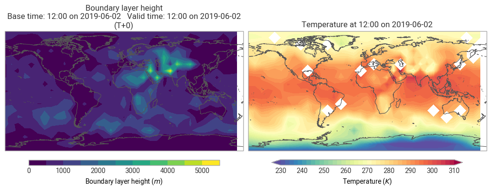
The target height in interpolate_pressure_to_height_levels() can also be a field/fieldlist, with changing target in each gridpoint. To demonstrate this we interpolate the temperature to the height of the boundary layer. First, we fetch the boundary layer height field for the same date and time as our input data.
[14]:
blh = ekd.from_source("sample", "blh_global.grib1").to_fieldlist()[0]
blh.ls()
[14]:
| parameter.variable | time.valid_datetime | time.base_datetime | time.step | vertical.level | vertical.level_type | ensemble.member | geography.grid_type | |
|---|---|---|---|---|---|---|---|---|
| 0 | blh | 2019-06-02 12:00:00 | 2019-06-02 12:00:00 | 0 days | 0 | surface | 0 | regular_ll |
This field contains heights above ground, so we need to set h_reference="ground" for the interpolation.
[15]:
t_res_blh = vertical.interpolate_pressure_to_height_levels(
    t,
    blh,
    z,
    zs=zs,
    h_type="geometric",
    h_reference="ground",
    interpolation="linear",
)
t_res_blh.ls()
[15]:
| parameter.variable | time.valid_datetime | time.base_datetime | time.step | vertical.level | vertical.level_type | ensemble.member | geography.grid_type | |
|---|---|---|---|---|---|---|---|---|
| 0 | t | 2019-06-02 12:00:00 | 2019-06-02 12:00:00 | 0 days | 637.9435 | height_above_ground_level | 0 | regular_ll |
We plot the boundary layer height and the temperature interpolated to it side by side.
[16]:
ekp.quickplot(ekd.FieldList.from_fields([blh, t_res_blh]))
[16]:
<earthkit.plots.components.figures.Figure at 0x13e32d220>
Writing to GRIB
Currently, fieldlist based computations resulting in fieldlist keeping all the values in memory. We can save this data to GRIB with to_target.
[17]:
t_res.to_target("file", "_pl_to_hl.grib")

# read back and verify
t_res_saved = ekd.from_source("file", "_pl_to_hl.grib").to_fieldlist()
t_res_saved.ls()
[17]:
| parameter.variable | time.valid_datetime | time.base_datetime | time.step | vertical.level | vertical.level_type | ensemble.member | geography.grid_type | |
|---|---|---|---|---|---|---|---|---|
| 0 | t | 2019-06-02 12:00:00 | 2019-06-02 12:00:00 | 0 days | 1000 | height_above_ground_level | 0 | regular_ll |
| 1 | t | 2019-06-02 12:00:00 | 2019-06-02 12:00:00 | 0 days | 5000 | height_above_ground_level | 0 | regular_ll |
[18]:
# the first 2 values from the saved fields
t_res_saved.values[:, :2]
[18]:
array([[269.52911377, 269.52911377],
       [249.74256897, 249.74256897]])
[ ]: